Satellite altimetry is definitely not my department, but I find it truly amazing what it can tell us about ocean currents. At its simplest a satellite measures how much the sea surface departs from the local horizontal for this determines the pressure field that balances the velocity field. Consider this, the sea level difference across the Gulf Stream in the previous post is about 1.2 m yet the satellite measures this to O(0.01) m resolution while orbiting Earth at 7.2 km/sec at 1337 km elevation! If that isn’t enough, the raw sea level measurement must be corrected for atmospheric water vapor and the electrical conductivity of the ionosphere for both affect the round-trip travel time for the satellite radar signal. On top of that corrections must be made for sea surface roughness and sea level change due to variations atmospheric pressure (when pressure goes up, sea level goes down – pushed toward lower pressure areas).
For the altimeter measurements to be useful, we also need to know the shape of our planet for it is not a simple sphere or ellipse. Due to varying mass distributions in the crust, the free surface, what is called the geoid, varies in elevation by more than 100 m. This figure shows what the geoid looks like for the Slope region and Bermuda. The black line denotes the 1000 m isobath along the continental slope. Note the 2 m contouring.
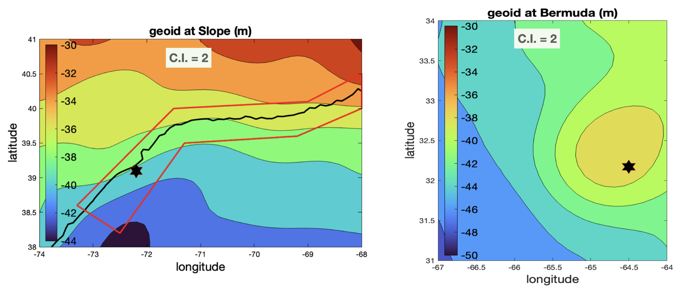 Due to the large change in depth between the shelf and Slope waters and hence mass distribution, the free surface varies some 10 m across the region. Similarly, the Bermuda seamount draws water toward it raising the sea level around the island by several meters. Lastly, we also need to know where the surface would be if the ocean were put to rest. Since we can’t do that the next best thing is to use all available data, velocity from floats, surface drifters, and current meter records to determine the mean surface velocity field. The balancing free surface elevation or mean ADT tells us how much it is deviating from where it would be if the ocean were at rest. The second figure shows the mean ADT across the Slope region and Bermuda with 0.2 and 0.02 m range for the two areas. The difference in mean ADT between the stars is 0.787 m. It is about 0.05 m too large, see below.
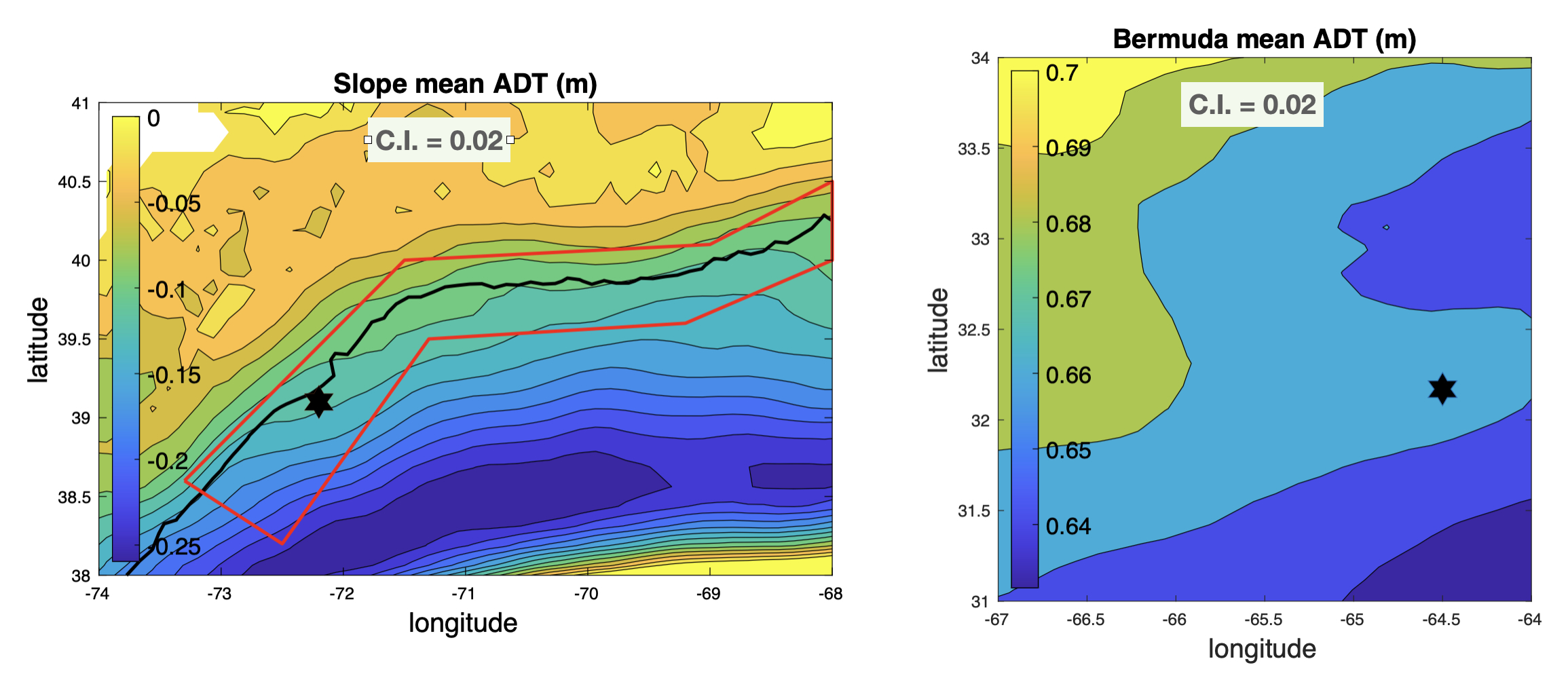
In the previous post where we estimated the depth of the level of zero transport three different ways, the estimate using mean ADT and Argo hydrography put the LZT nearly 200 m deeper than the two other estimates. I suspect the reason due to uncertainties in the contouring of the mean ADT field along the continental slope where there are strong gradients in both the geoid and the mean surface circulation. Particularly suspicious are the mean ADT contours SW of 40°N 71°W crossing the 1000 m isobath toward the shelf. This is an area where the mean flow should along the slope or possibly a bit off shelf since all water must be forced off the shelf where it narrows north of Cape Hatteras.
To bring the black transport curve in the previous post into alignment with the other two estimates, i.e. to the green curve, would require reducing the Slope-Bermuda ADT difference by about 0.05 m. While it is only the difference that matters, most of the correction should probably be applied to Slope with its large cross-slope gradient. but the relationship of mean ADT between Bermuda and Slope also depends upon the accuracy of the mean surface velocity field between the two. Getting this right is not a trivial exercise due to a vigorous seasonal cycle of winds, temperature and precipitation across the region.
The uncertainties in the mean ADT notwithstanding, ADT is an incredibly powerful for mapping surface currents. Please visit this website:
https://currents.soest.hawaii.edu/oleander/vel_ssh_quick/index.html
It shows the Oleander surface velocity vectors superimposed on the concurrent map of surface ADT from Copernicus Marine Service. These figures show how vessels in repeat traffic can work together with altimetry to a) provide spatial context, b) ground truth about the inferred surface velocity field and most importantly, c) to extend our vision into the water column. Even if we knew the dynamic height profiles throughout the ocean (which we don’t due to the large spatial and temporal separation between Argo float profiles), we wouldn’t be able to construct a dynamic height field accurate enough to give useful information about the weaker currents at depth. That is what has made the sustained ADCP observations on the Oleander, the Explorer of the Seas, Nuka Arctica, Norröna, and the Laurence M. Gould so incredibly useful. The point is that a single ADCP on these vessels, operating 24/7 on repeat routes for years on end, has opened up horizontal-vertical-time domains for study that cannot be explored with any of our traditional oceanographic methods.