As I mentioned earlier, the Pegasus program spanned the years 1980-1983 during which time we mapped the velocity field of the Gulf Stream roughly every two months. The primary objective was to directly measure how much water was being transported by the current. This was a big step forward for until then all estimates of transport were geostrophic (determining the pressure field from hydrography and assuming a zero reference velocity at great depth). We knew this was unsatisfactory, but what else could we do? The April 19, 2025 blog-post has the details of the Pegasus program. A little later I started looking more closely at the vertical structure of the current. The approach was to decompose the velocity field into what are known as normal modes. These are theoretical descriptions of how the water column can move over a flat bottom ocean given its density (temperature/salinity) structure. The normal modes can be viewed either as vertical displacements of the density field or as horizontal velocity modes, we work with the latter here. The results were quite striking (Rossby, 1987).
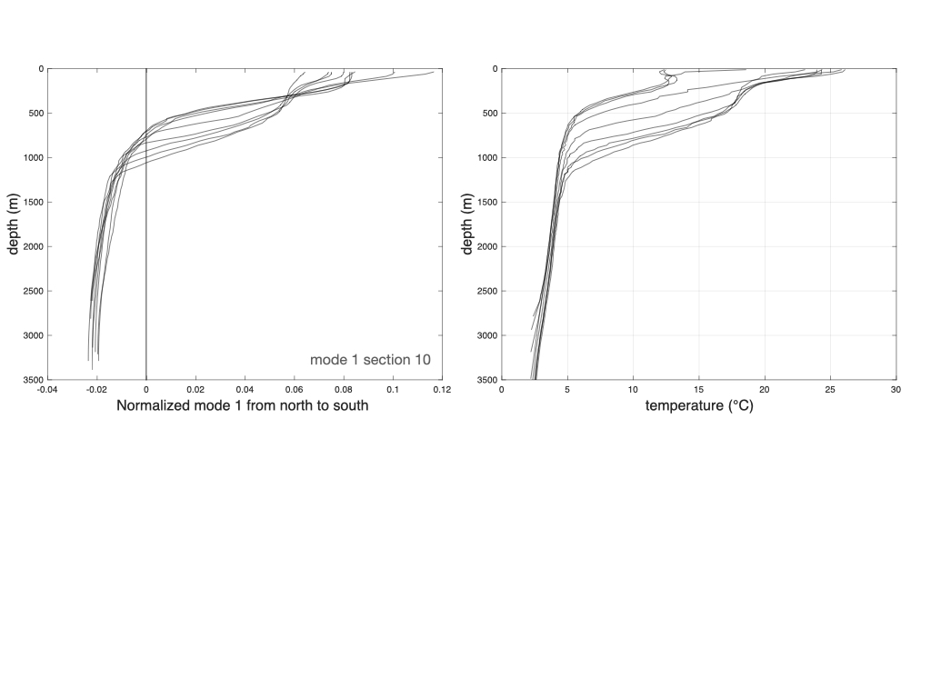
We know much more about these things today, but at the time I was surprised at the findings. What must be mentioned here is that the normal modes describe the vertical structure of the current, the modes have zero vertically-averaged velocity. Transport is accounted for with a depth-independent mode, what we call the barotropic mode with the mode designation 0. This will become clear in the figures. While the results are rather general, I’ll just show an example from the Gulf Stream. The first figure shows mode 1 for the 9 sites across the Gulf Stream (left panel). You can see that it is a smoothed simulacrum of the corresponding temperature profiles (right panel). Although some details go missing the key thing is that as the temperature profile deepens, so does the zero crossing of the modes.
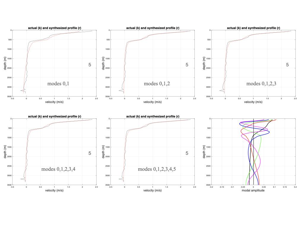
The second figure shows downstream velocity at site 5 from section 20. The black line shows the observed velocity profile while the red line in the five panels shows the synthesized profile using mode 0 and mode 1 in the first panel, modes 0,1,2 in the second panel etc. The five panels show how effectively just mode 0 and 1 account for the observed profile. Including mode 2 helps a little bit, but adding in modes 3,4, and 5 leads to little further improvement. The bottom right shows what the first 5 modes look like. Mode 1 has one zero crossing (k), mode 2 has two zero crossings (r), each of the higher modes add an additional zero crossing (g, b, and m, resp.). One can go to higher and higher modes, but each of these will contribute only infinitesimally to the synthesis.
There is rough equipartition of kinetic energy between modes 0 and 1 (mode 1 slightly greater) with very little present in the higher ones. Modes 0 and 1 account for more than 90% in the kinetic energy in the profile! Outside the stream the total kinetic energy is of course much less, but the lowest modes still suffice to account for the structure of the profile. Since the velocity profiles have been rotated into a down- and cross-stream directions, it follows that there is little structure to the cross-stream profile. But the residual kinetic energy (what is left distributed across the higher modes) is virtually the same in both directions. We can’t determine its temporal properties, but most likely it reflects internal wave motion including inertial oscillations. That these normal modes work so efficiently to describe the velocity profile depends upon knowing the concurrent stratification, as indicated in the first figure.
Rossby, T. (1987). On the energetics of the Gulf Stream at 73o W. J. Mar. Res., 45, 59-82.